
Anna-Lena Popkes
Saturday, February 2, 2019
Kullback-Leibler Divergence
One of the points on my long ‘stuff-you-have-to-look-at’ list is the Kullback-Leibler divergence. I finally took the time to take a detailed look at this topic.
Definition
The KL-divergence is a measure of how similar (or different) two probablity distributions are. When having a discrete probability distribution $P$ and another probability distribution $Q$ the KL-divergence for a set of points $X$ is defined as:
$$D_{KL}(P ,|| ,Q) = \sum_{x \in X} P(x) \log \big( \frac{P(x)}{Q(x)} \big)$$
For probability distributions over continuous variables the sum turns into an integral:
$$ D_{KL}(P ,|| ,Q) = \int_{-\infty}^{\infty} p(x) \log \big( \frac{p(x)}{q(x)} \big) dx$$
where $p$ and $q$ denote the probability density functions of $P$ and $Q$.
Visual example
The Wikipedia entry on the KL divergence contains a nice illustration:
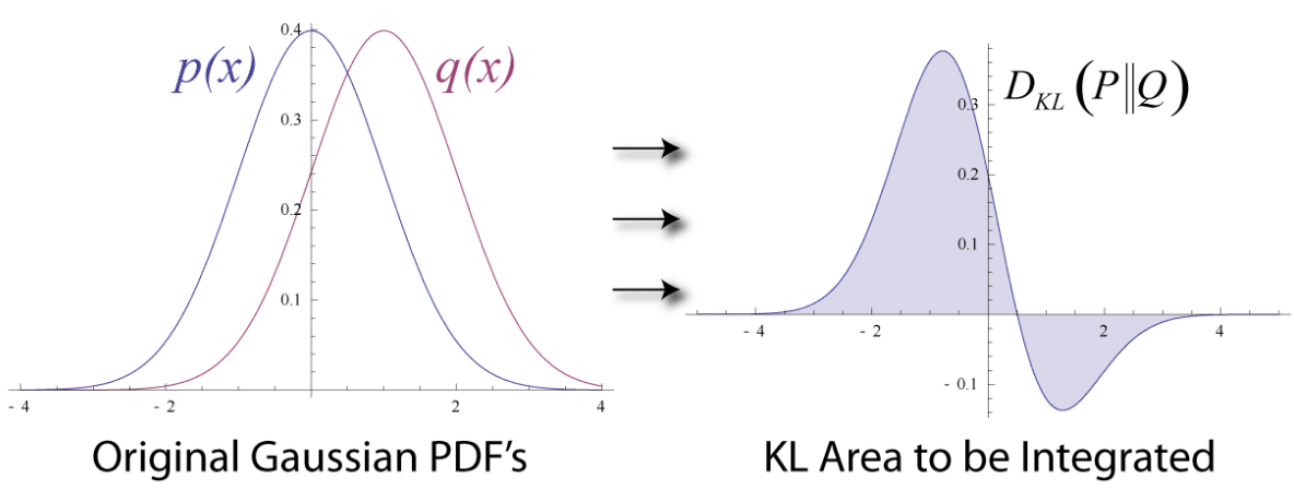
On the left hand side we can see two Gaussian probability density functions $p(x)$ and $q(x)$. The right hand side show the area that is integrated when computing the KL divergence from $p$ to $q$. We know that:
$$ \begin{align} D_{KL}(P ,|| ,Q) &= \int_{-\infty}^{\infty} p(x) \log \big( \frac{p(x)}{q(x)} \big) dx \ &= \int_{-\infty}^{\infty} p(x) \big( \log p(x) - \log q(x) \big) dx \end{align} $$
So for each point $x_i$ on the x-axis, we compute $\log p(x_i) - \log q(x_i)$ and multiply the result by $p(x_i)$. We then plot the resulting y-value in the right hand plot. This is how we get to the curve given in the right hand plot. The KL divergence is now defined as the area under the graph, which is shaded.
KL divergence in machine learning
In most cases in machine learning we are given a dataset $X$ which was generated by some unknown probability distribution $P$. In this approach $P$ is considered to be the target distribution (that is, the ’true’ distribution) which we are trying to approximate using a distribution $Q$. We can evaluate candidate distributions $Q$ using the KL-divergence from $P$ to $Q$. In many cases, for example in variational inference, the KL divergence is used as an optimization criterion which is minimized in order to find the best candidate/approximation $Q$.
Interpreting the Kullback Leibler divergence
Note: Several different intepretations of the KL divergence exist. This interpretation describes a probabilistic perspective which is often useful for machine learning.
Expected value
In order to understand how the KL divergence works, remember the formula for the expected value of a function. Given a function $f$ with $x$ being a discrete variable, the expected value of $f(x)$ is defined as
$$\mathbb{E}\big[f(x)\big] = \sum_x f(x) p(x)$$
where $p(x)$ is the probability density function of the variable $x$. For the continuous case we have
$$\mathbb{E}\big[f(x)\big] = \int_{-\infty}^{\infty}f(x) p(x) dx$$.
Example: Suppose you made a very good deal and bought three pairs of the best headphones for a reduced price of 200 USD each. You want to sell them for 350 USD each. We define the probability of selling $X=0, X=1, X=2, X=3$ headphones as follows:
$$p(X=0) = 0.1$$ $$p(X=1) = 0.2$$ $$p(X=3) = 0.3$$ $$p(X=4) = 0.4$$
We further define a function that measures profit: $f(x) = \text{revenue} - \text{cost} = 350*X - 200*X$. For example, when selling two pairs of headphones you will make: $f(X=2) = 700 - 400 = 300$. So what’s our expected profit? We can compute it using the formula for the expected value:
$$
\begin{align}
\mathbb{E}\big[f(x)\big] &= p(X=0)*f(X=0) + p(X=1)*f(X=1) + p(X=2)*f(X=2) + p(X=3)*f(X=3) \\
&= 0.1 * 0 + 0.2 * 150 + 0.3 * 300 + 0.4 * 450 \\
&= $ 300
\end{align}
$$
Ratio of p(x) / q(x)
Looking back at the definition of the KL divergence we can see that it’s quite similar to the definition of the expected value. When setting $f(x) = \log \big(\frac{p(x)}{q(x)}\big)$ we can see that:
$$ \begin{align} \mathbb{E}\big[f(x)\big] &= \mathbb{E}_{x \sim p(x)}\big[\log \big(\frac{p(x)}{q(x)}\big) \big] \\ &= \int_{-\infty}^{\infty} p(x) \log \big( \frac{p(x)}{q(x)} \big) dx \\ &= D_{KL}(P || Q) \end{align} $$
But what does that mean? Let’s start by looking at the quantity $\frac{p(x)}{q(x)}$. When having some probability density function $p$ and another probability density function $q$ we can compare the two by looking at the ratio of the two densities:
$$ratio = \frac{p(x)}{q(x)}$$
Insight: We can compare two probability density functions by means of the ratio.
Because both $p(x)$ and $q(x)$ are probability densities they output values between $0$ and $1$. When $q$ is similar to $p$, $q(x)$ should output values close to $p(x)$ for any input $x$.
Example: For some input $x_i$, $p(x_i)$ might be 0.78, i.e. $p(x_i) = 0.78$. Let’s look at different densities $q$:
a) If $q$ and $p$ are identical, $q(x)$ would output the same value and the resulting ratio would be one:
$ratio = \frac{p(x)}{q(x)} = \frac{0.78}{0.78} = 1$
b) When $q(x)$ assigns a lower probability to the input $x$ than $p(x)$, the resulting ratio will be larger than one:
$ratio = \frac{p(x)}{q(x)} = \frac{0.78}{0.2} = 3.9$
c) When $q(x)$ assigns a higher probability to the input $x$ than $p(x)$, the resulting ratio will be smaller than one: $$ratio = \frac{p(x)}{q(x)} = \frac{0.78}{0.9} \approx 0.86$$
The example provides an important insight:
Insight: For any input $x$ the value of the ratio tells us how much more likely $x$ is to occur under $p(x)$ compared to $q(x)$. A value of the ratio larger than 1 indicates that $p(x)$ is the more likely model. A value smaller than 1 indicates that $q$ is the more likely model.
Ratio for entire dataset
If we have a whole dataset $X = x_1, …, x_n$ we can compute the ratio of the entire set by taking the product over the individual ratios. Note: this only holds if the examples $x_i$ are independent of each other.
$$ratio = \prod_{i=1}^n \frac{p(x_i)}{q(x_i)}$$
To make the computation easier we can take the logarithm:
$$\text{log_ratio} = \sum_{i=1}^n \log \big( \frac{p(x_i)}{q(x_i)} \big)$$
When taking the logarithm, a log ratio value of 0 indicates that both models fit the data equally well. Values larger than 0 indicate that $p$ is the better model, that is, it fits the data better. Values smaller than 0 indicate that $q$ is the better model:
Example calculation
Let’s calculate the KL divergence for our headphone example. We already have specified a distribution $P$ over the possible outcomes. Let’s define another distribution $Q$ which expresses our belief that it’s very likely that we sell all three pairs of headphones and less likely that we don’t sell all of them (or none).
| Distribution | $X = 0 \quad$ | $X=1 \quad$ | $X=2 \quad$ | $X=3 \quad$ |
|---|---|---|---|---|
| $P(X)$ | 0.1 | 0.2 | 0.3 | 0.4 |
| $Q(X)$ | 0.1 | 0.1 | 0.1 | 0.7 |
How similar are $P$ and $Q$? Let’s compute the KL divergence: $$ \begin{align} D_{KL}(P || Q) &= \sum_{x \in X} P(x) \log \big( \frac{P(x)}{Q(x)} \big) \\ &= 0.1 * \log \big( \frac{0.1}{0.1} \big) + 0.2 * \log \big( \frac{0.2}{0.1} \big) + 0.3 * \log \big( \frac{0.3}{0.1} \big) + 0.4 * \log \big( \frac{0.4}{0.7} \big) \\ &\approx 0.244 \end{align} $$
Ratio vs. KL-divergence
We discovered that the log-ratio can be used to compare two probabilty densities $p$ and $q$. The KL divergence is nothing else than the expected value of the log-ratio. When setting $f(x) = \log \big(\frac{p(x)}{q(x)}\big)$ we receive:
$$ \begin{align} \mathbb{E}\big[f(x)\big] &= \mathbb{E}_{x \sim p(x)}\big[\log \big(\frac{p(x)}{q(x)}\big) \big] \\ &= \int_{-\infty}^{\infty} p(x) \log \big( \frac{p(x)}{q(x)} \big) dx \\ &= D_{KL}(P || Q) \end{align} $$
Insight: The KL divergence is simply the expected value of the log-ratio of the entire dataset.
Why is the KL divergence always non-negative?
An important property of the KL divergence is that it’s always non-negative, i.e. $D_{KL}(P , || , Q) \ge 0$ for any valid $P, Q$. We can prove this using Jensen’s inequality.
Jensen’s inequality states that, if a function $f(x)$ is convex, then
$$\mathbb{E}[f(x)] \ge f(\mathbb{E}[x])$$
To show that $D_{KL}(P , || , Q) \ge 0$ we first make use of the expected value:
$$ \begin{align} D_{KL}(P || Q) &= \int_{-\infty}^{\infty} p(x) \log \big( \frac{p(x)}{q(x)} \big) dx \\ &= \mathbb{E}_{x \sim p(x)}\big[\log \big(\frac{p(x)}{q(x)}\big) \big] \\ &= - \mathbb{E}_{x \sim p(x)}\big[\log \big(\frac{q(x)}{p(x)}\big) \big] \end{align} $$
Because $-\log(x)$ is a convex function we can apply Jensen’s inequality:
$$ \begin{align} -\mathbb{E}_{x \sim p(x)}\big[\log \big(\frac{q(x)}{p(x)}\big) \big] &\ge - \log \big( \mathbb{E}_{x \sim p(x)}\big[\frac{q(x)}{p(x)} \big] \big) \\ &= - \log \big( \int_{-\infty}^{\infty} p(x) \frac{q(x)}{p(x)} dx \big) \\ &= - \log \big( \int_{-\infty}^{\infty} q(x) dx \big) \\ &= - \log(1) \\ &= 0 \end{align} $$
Which type of logarithm to use
It’s interesting to note that we can use different bases for the logarithm in the definition of the KL divergence, depending on the interpretation. For example, when using the natural logarithm the result of the KL divergence is measured in so called ’nats’. When using the logarithm to base 2 the result is measured in bits.